Using Nested List Comprehensions to Serialize Python Objects

A common pattern in building RESTful web services is the serialization of internal state into a JSON structure for transmission.  Writing this serialization in a way that is clear and easy to understand helps improve code quality and maintainability.  Using Python’s list comprehension can help us achieve these aims.

For the purposes of this article, let us consider a simple toy example.  We’ll create an “Order” object that can be populated with “Inventory” items.  In our response we’ll want to publish a JSON object listing of all our orders and the items in each order that were ordered for express delivery.

from typing import List
from uuid import uuid4
 
# Sample classes for building our data structure
class Inventory:
    def __init__(self, name: str, express: bool=False):
        self.name = name
        self.express = express
        self.id = str(uuid4())
 
class Order:
    def __init__(self, first: str, last: str, items: List[Inventory]):
        self.first = first
        self.last = last
        self.items = items
        self.id = str(uuid4())
 
# Build a sample data set
orders = [
    Order('John', 'Smith', [
        Inventory('Apple', True),
        Inventory('Sausage'),
        Inventory('Eggs')
    ]),
    Order('Hildred', 'Spencer', []),
    Order('Candice', 'Silvester', [
        Inventory('Ham', True),
        Inventory('Potato', True)
    ]),
]

To serialize this structure into a JSON response there are a number of ways we could approach the problem.  Let us first consider how we might build this out piece by piece. In this first example we first iterate over the list of orders. Then we will iterate over the items in the order adding serializations if the item is ordered with express delivery. With that complete we then serialize the order and add it to the list of serialized orders. This code is perfectly functional, but the structure of our serialization is hidden among the logic statements. How might we go about improving readability of this code?

order_list = []
for order in orders:
    items = []
    for item in order.items:
        if item.express:
            item_status = {
                'id': item.id,
                'name': item.name,
            }
            items.append(item_status)
    order_status = {
        'name': ' '.join((order.first, order.last)),
        'id': order.id,
        'items': items,
    }
    order_list.append(order_status)
status = {
    'orders': order_list,
}

We can start by using a list comprehension to simplify our loop for building the item list. This collapses the inner loop down in to a single line.

order_list = []
for order in orders:
    items = [{'id': item.id, 'name': item.name} for item in order.items if item.express]
    order_status = {
        'name': ' '.join((order.first, order.last)),
        'id': order.id,
        'items': items,
    }
    order_list.append(order_status)
status = {
    'orders': order_list,
}

However, we can keep going by creating a nested list comprehension to subsume the outer loop as well.  Doing so allows us to simplify further.  Now if we were simply concerned about line count, this could reduce our serialization down to just a few lines. However, readability and line length matter as well. So instead, let’s expand the list comprehension across multiple lines to create our final serialization code.  A complete copy of the final code is available as a gist here.

status = {
    'orders': [
        {
            'name': ' '.join((order.first, order.last)),
            'id': order.id,
            'items': [
                {
                    'name': inventory.name,
                    'id': inventory.id,
                }
            for inventory in order.items if inventory.express  # Nested list comprehension with conditional statement
            ]
        }
        for order in orders  # Simple list comprehension to iterate over the orders in the list
    ]
}

It should now be clearly obvious to any reader what the structure of our JSON object is. If we compare this code to the JSON it generates, we can see how they visually resemble each other.

{
    "orders": [
        {
            "name": "John Smith",
            "id": "7e5369c2-a8af-4205-becc-6c05dde7bf2c",
            "items": [
                {
                    "id": "d7f14359-a758-46b3-8ba0-cd515daf6c32",
                    "name": "Apple"
                }
            ]
        },
        {
            "name": "Hildred Spencer",
            "id": "b5d413a8-ac24-43a7-8b12-6ee5c0a34cd2",
            "items": []
        },
        {
            "name": "Candice Silvester",
            "id": "eea4d01a-334f-4259-a0e2-8f5879684a25",
            "items": [
                {
                    "id": "52040e4d-1cb3-47ab-b9d4-d7959ce10d00",
                    "name": "Ham"
                },
                {
                    "id": "e68e0a7c-7092-47e1-b3bc-e04d113ab446",
                    "name": "Potato"
                }
            ]
        }
    ]
}

Using list comprehensions like this can help us express the creation of data structures in a way that is natural and clean.  This example focused on creating a dictionary for consumption by a JSON serializer, but the principal can be applied to many other cases.  Consider the creation of a nested structure of objects such as the sample data set used in this example.  How might we have constructed it had we been given another data structure, such as JSON perhaps, to generate it?  Are there places in your code where this could be applicable?
UAV CMOS Distortion

Using unmanned vehicles to capture aerial images is likely the most common use for these platforms.  The imaging system on these vehicles often uses a CMOS image sensor thanks to their relatively low-cost and wide spread use in most DSLR cameras.  One challenge of these sensors is that they can be susceptible to rolling shutter distortion.  The final result can vary between an image distorted beyond any usability and being imperceptible.

Webcam

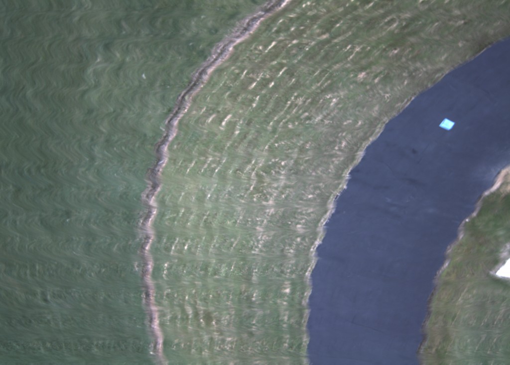
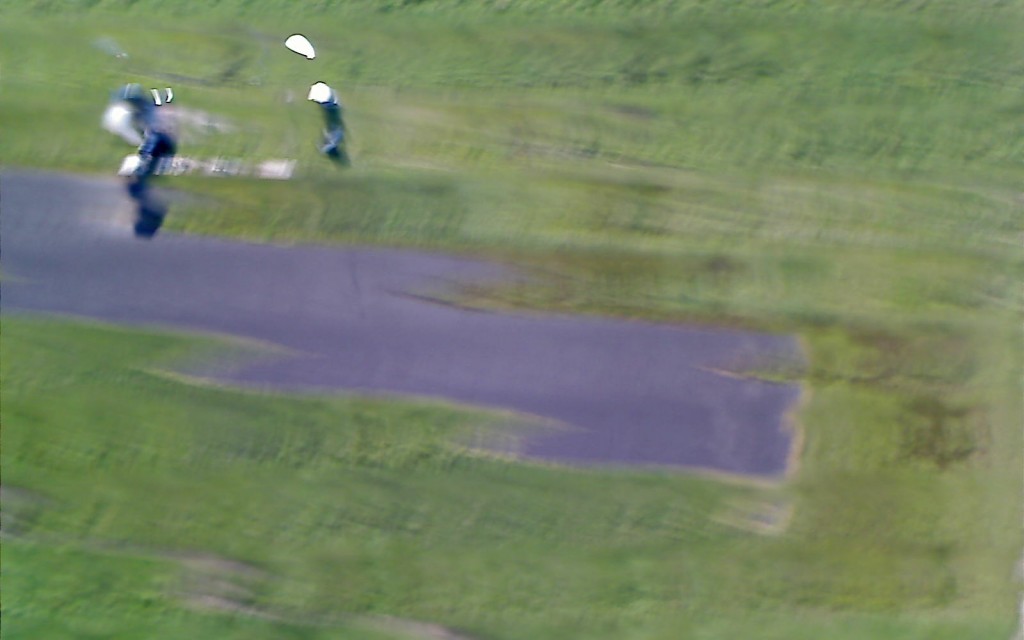
In this first example a Logitech Webcam Pro 9000 was attach to a Beaglebone black which would continuously take snapshots.  The imagery system was mounted on a 25 pound fixed wing aircraft with a gas engine.  From the photo it is clear that, due to the slowness of the capture, the image is largely unusable.

Bad distortion from web camera

Bad distortion from web camera.


Go-Pro

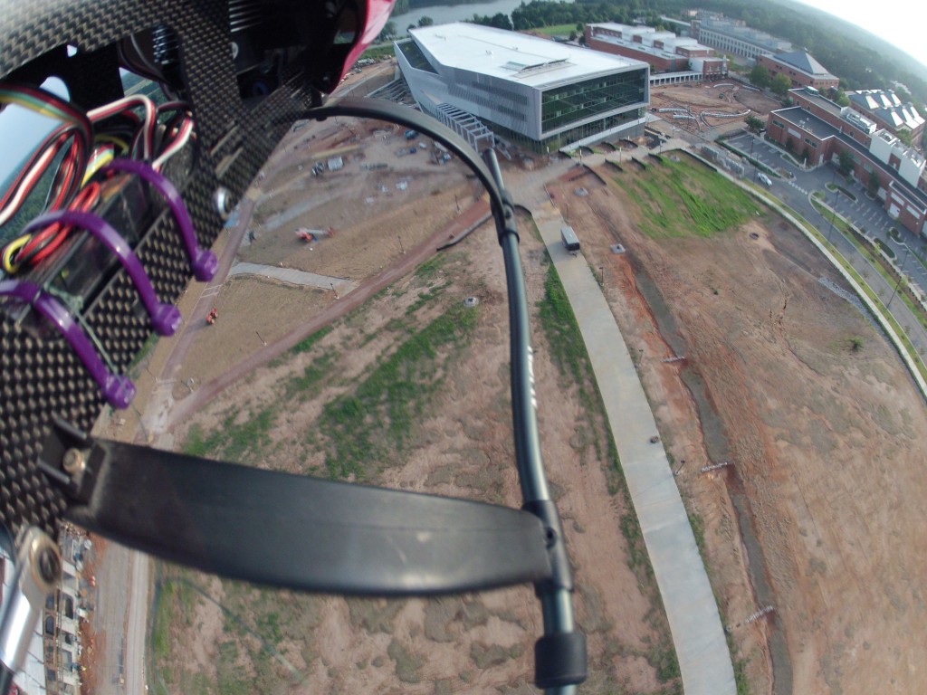
In another experiment a GoPro was mounted to the side of an electric helicopter.  The image here is much more usable and the distortion may not even be obvious with the exception of the landing gear in the foreground.  This highlights one of the dangers of this kind of distortion.  While the distortion may sometimes be very obvious, it may also be very subtle in the image.


Go-Pro mounted on a helicopter showing CMOS distortion on the landing gear


IDS Camera

While the camera and its settings play an important role in determining the effect of rolling shutter, the mount and vehicle dynamics can also have a dramatic effect.  In this case, the same camera with similar settings was mounted on a gas powered helicopter and then a gas powered fixed wing aircraft.

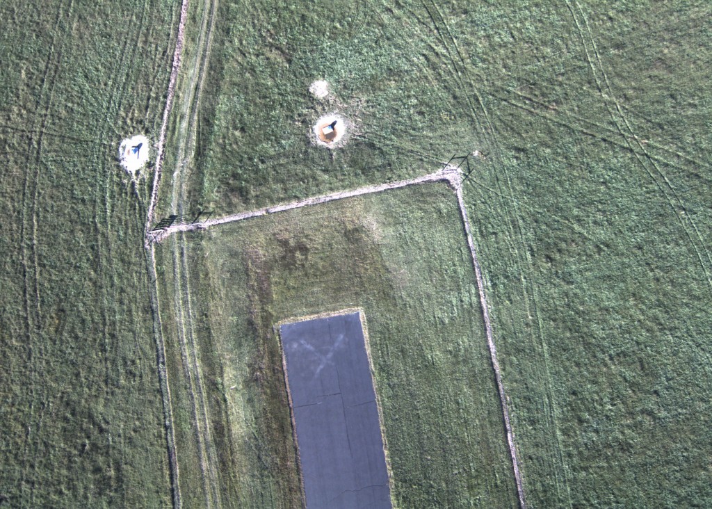
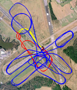
The helicopter was then flown through an aggressive set of maneuvers will the camera was capturing photos.  The camera was mounted directly to the helicopter frame with minimal vibration damping.  In the image there are two sources of distortion obvious.  Firstly, the straight runway now appears to arc up to the right.  This is a result of the rapid yawing of the helicopter during the capture.  The second source of distortion is obvious in the grass, fence, and edges of the photo.  This higher frequency distortion is a result of the helicopter vibration as a result of the rotor.

Helicopter Test

When the camera was mounted to the fixed-wing aircraft, the image that is captured is substantially better.  There is no obvious distortion as a result of the rolling shutter.  The slower dynamics of the fixed wing aircraft flying straight, level, and steady keep the runway straight.  The lower vibration levels of the aircraft and the addition of a vibration isolated mount removes the second source of distortion.  It bears mentioning that differences in the color quality of the image may also be influenced by difference in sunlight between the two flights.

IDS Camera mounted on a fixed wing aircraft

The effects of rolling shutter on aerial imagery can be quite severe, but are not insurmountable.  Being conscious of these effects can help of when evaluating the camera hardware, sensors, mounting and vehicle dynamics which all feed into determining the final quality of the image.

Matlab Central

The Aerospace Design Toolbox is now available on Matlab Central.  This release includes examples on how to use the various functions to integrate with XFoil, AVL, and more.

Aerospace Design Toolbox

I’ve recently switched to using Github for my open source projects.  As apart of this transition, I’ve been restructuring some of my old code.  This has lead to the creation of the aerospace-design-toolbox (ADT).

This Matlab toolbox is built from the Mavl code base.  The biggest difference between the two is scope.  While Mavl was designed to address the full scope of the design process from modeling to analysis, the ADT simply supports loading data from other aerospace software into Matlab.  Currently the ADT reads output files from AVL and Xfoil.  It can additionally read prop data in the format used by the UIUC propeller database.  For more information on what is and isn’t supported please see the README.m file in the repository.

At this time the toolbox is just a set of utility functions.  In the near term development will focus on converting the code into a standard toolbox that will integrate better with Matlab.

AUVSI USUAS – NCSU Aerial Robotic Club 2012 Resuts

The following details the mission performance of NC State University’s Aerial Robotics Club at the 10th annual AUVSI Student Unmanned Systems competition.

The autopilot successfully executed a fully autonomous take-off before switching over to manual control due to an error in the autopilot’s altitude configuration.  It was later determined to have been operator error caused by improper zeroing of the altitude.  Autonomous control was regained by flying at a higher altitude than originally planned.  The waypoints, search pattern, and emergent target pattern were flown at this fixed altitude.

One special feature added this year was a laser altimeter.  Despite early concerns of a failure, the altimeter performed well through out the mission.

The SRIC message was determined to be:

John Paul Jones, defeated British ship Serapis in the Battle of Flamborough Head on 23 September 1779

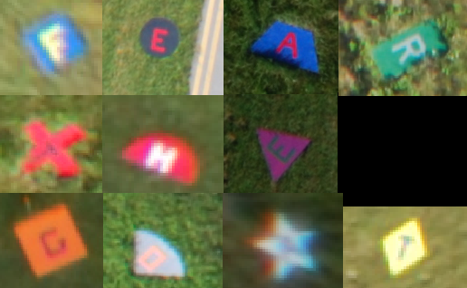
The targets this year spelled out the phrase, “Fear the goat”.  This apparently has something to do with the mascot of the United States Naval Academy “Bill the goat”.

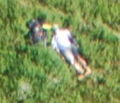
The emergent target this year was a wounded hiker and his backpack.  Most of these details were visible in the images taken with the exception of his wounds.

2012 AUVSI USUAS Results

The 10th annual Undergraduate Student Unmanned Aerial Systems competition hosted by AUVSI’s seafarer chapter concluded last week.  Teams from across the United States, Canada, India, and Turkey converged on Webster naval airfield for several days of autonomous competition.

Final standings

  1. Universite de Sherbrooke
  2. Embry-Riddle (UARE)
  3. California State at Northridge
  4. Delhi Technical University
  5. Cornell University
  6. North Carolina State University
Best Journal – University of Texas at Austin
Best Oral Brief – Kansas State University
Best Mission – Universite de Sherbrooke

 Autopilots

Listed here are some of the autopilots used by various schools.  If you know what autopilots any other schools were using please comment below.

Piccolo

  • North Carolina State University
  • Mississippi University
  • Kansas State University
  • Kansas State University (Pomona)
  • Cornell University
  • New Delhi University

Papparazzi

  • Universite de Sherbrooke
Micropilot
  • Great Mills High School
Custom
  • Utah State (Rotary)

Ardupilot

  • Rutgers University
  • Embry Riddle Prescott

3D Laser Cutting With a 2D System

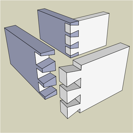
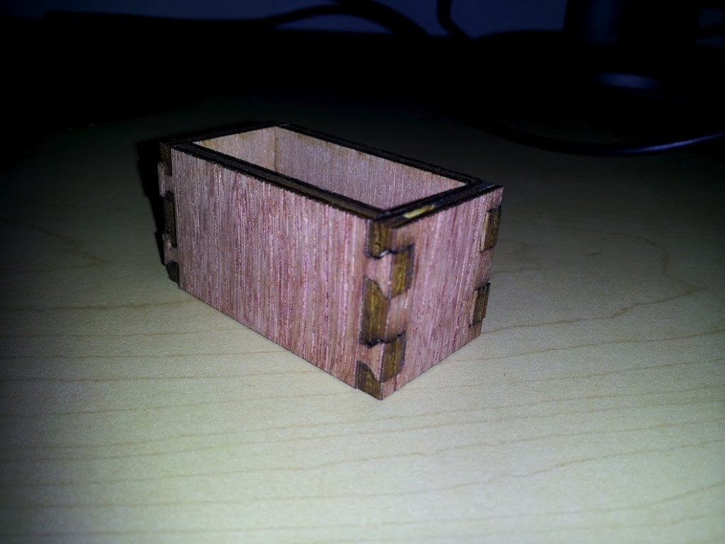
A typical laser cutter can make a precise 2D cut.  With rastering it is possible to etch the surface to add labeling.  However if the power of the laser can be finely controlled it is possible to make engineered depth cuts such as trenches or angled slopes.  This allows for laser cutting complex geometries such as a dovetail joint.

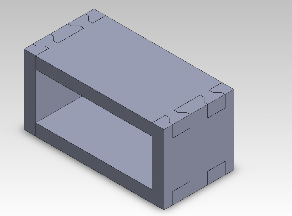
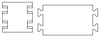
For this experiment a simple dovetail jointed box was modeled in Solidworks.

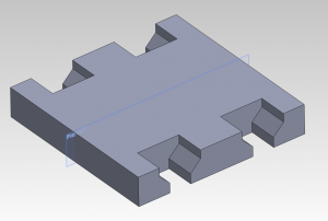
Although the long size of the box can be cut using typical methods, the end plates cannot.

Both parts where placed into a solidworks drawing which was then exported to *.pdf.  This was then imported into Corel Draw 5.  The initial drawings appeared as shown below.

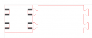
The lines to be cut were converted to “hairline” and RGB code <255,0,0>.  The Raster layer is defined by the gray-scale where back is 100% and white is 0%.  The power of the laser at 100% is set in the printer’s cut settings when the part is ready to be printed.  In this case, a gradient was drawn into the areas needing a depth cut.  The gradient allows for an angled cut between two particular depths.  The colors used and the number of passes to be completed were determined using a sort of look-up table.

Before this experiment, a set of colored squares were rastered into a material sample.  This was then repeated with two and three passses.  When selecting colors for the end plate cutting, the row that could reach the proper depth was selected.  In this case, the three-passes row was used with black at one end and a dark grey at the other.  This would result in a cut that was three black passes deep at one end and three dark-grey passes at the other.


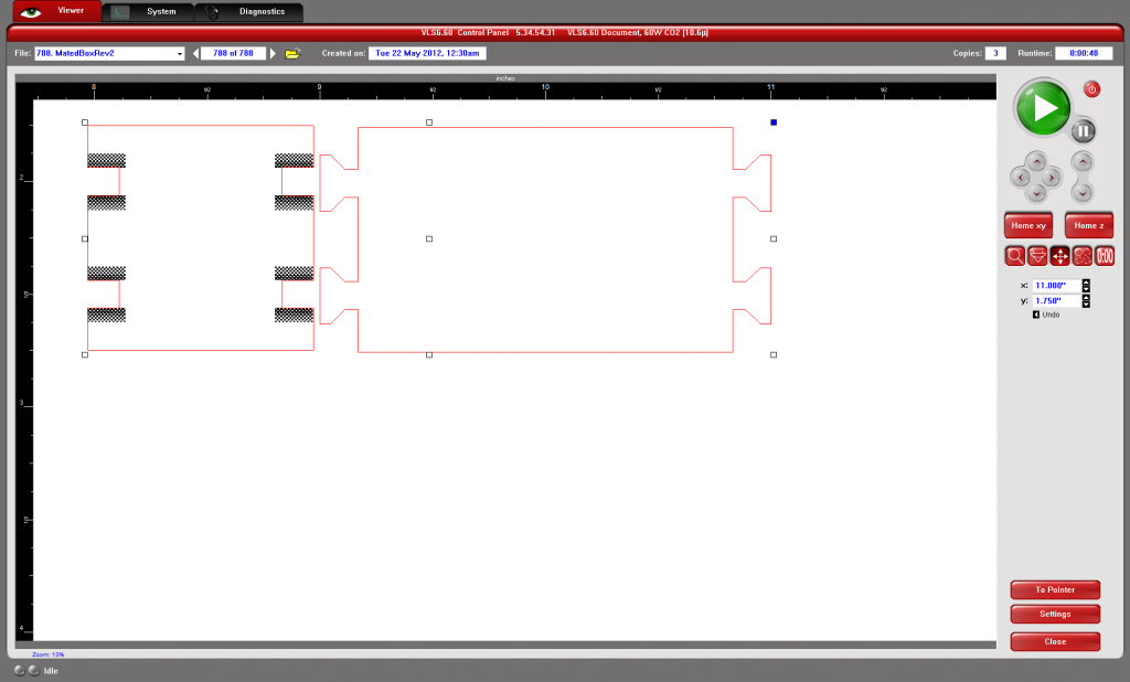
Shown in the laser cutting software below, the final design was then sent to the laser. For the first two passes, the vector cutting was set to be skipped.  This allowed the depth cutting to be finished before the laser cut out the final outline.

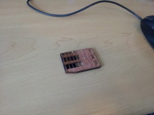
Finally the parts were removed from the laser cutter and the box shown below was assembled.  Two notable characteristics of the unglued box are its strength and its ease of assembly.  Even without glue the box doesn’t deform and tends to hold its shape.  Assembly was easier than just a tabbed box because once a joint was put together it had limited degrees of freedom about which to move.

Although this method can be time-consuming to setup, the final result creates good joints useful in engineered parts.

Servo Sin Wave

Automatic code generation is a powerful tool that when combined with Simulink promises important benefits to students and highly complicated applications alike.  Mathworks distributes an Arduino Blockset for Simulink.  The Arduino platform is a desirable to use because of its simple architecture and available hardware.  These hardware options include the ArdupilotMega (APM) which includes sensors and pinouts that will make it easier to integrate into a future aerial vehicle.

While the 2012a version only requires the base Matlab and Simulink packages, NCSU does not currently provide the 2012a version to students.  Instead the 2011a version was used since it was available.  It is not expected that there will be problems using the work done with 2011a in the 2012a release.

The base Arduino blockset includes blocks for Analog and Digital I/O as well as serial communication.  To take full advantage of the capabilites of the APM, additional blocks for SPI, I2C, PPM, and Servos are needed.  Development of a servo blocks has been the focus of this last week.

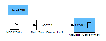
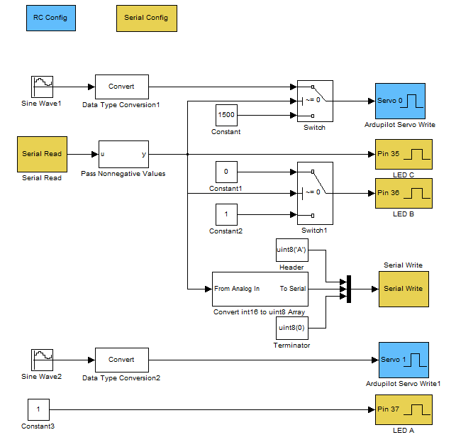
  The new blocks, shown in blue, allow for the configuration and control of servos attached to the APM.  An interesting note  is that although the APM only has 8 servo lines broken out on the side, there are an additional 3 lines (PL3, PB5, and PE3) that can be configured to output PWM commands. These lines are broken out from the APM base-board, but are not available on the sensor-shield “Oilpan”.

With just the blocks from the base, shown in yellow, and the new servo blocks it is already possible to access quite a few of the APM’s functions.  The demonstration program shown above commands two servos through a sin wave motion.  Data is read from the serial port allowing for the functionality of Servo 1 to be switched between sin wave and center position.

3D Printed Plug

In the process of manufacturing a senior design aircraft, a plug is used to create a negative mold on which aircraft fuselage skins can be laid up.  When the 2010-2011 senior design groups fabricated fuselage plugs, it was a lengthy process involving foam, plywood, fiberglass, epoxy, bondo, spackle, and an incredible amount of sanding.

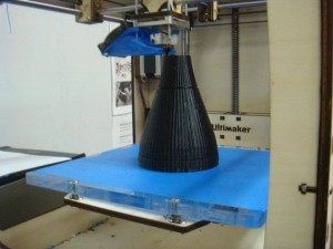
This year a new method was tried with the intent of reducing the time required to manufacture the plug and allow for more complex geometric shapes to be used.  The availability of cheap rapid prototyping machines made this possible.  For this experiment the Ultimaker 3D printer in the Entrepreneurship Garage was used.  Based on previous experiments, PLA was used as the printed material.  North Carolina State University’s Aerospace Engineering Senior Design teams 3 and 4 participated in the experiment and provided the labor to integrate the printed parts into their aircraft plugs.

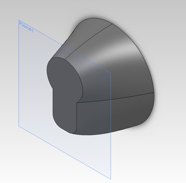
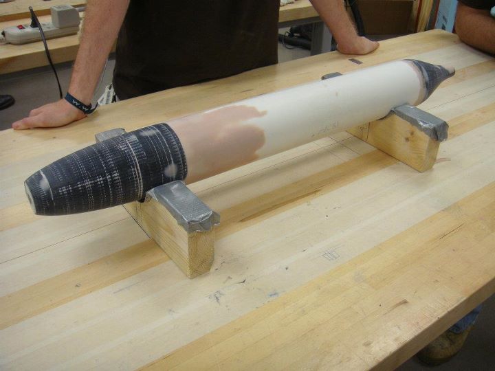
During the fall semester, the seniors designed the fuselage in solidworks.  The designs used a section of off-the-shelf PVC tubing as the main body with a nose cone and tail cone on either end to create the plug.  The nose and tail cones were modeled as separate parts and exported to *.STL format.

Team 3's Nose Cone

The UltireplicatorG software was then used to “slice” the model and create a GCODE instructions that the 3D printer could use.  In total, four parts were to be printed for the two teams.  Over the course of the printing a number of settings were experimented with.  The best results came when the solidworks models were simple solid objects with no shelling.  The slicer was then configured to print the object with zero infill and walls 3 layers thick.  This gave an object that was fast to print, but still rigid enough to be usable.  The final thickness of the wall was roughly 2-3 millimeters.

As this tail cone was being printed the extruder failed leaving several weak layers.

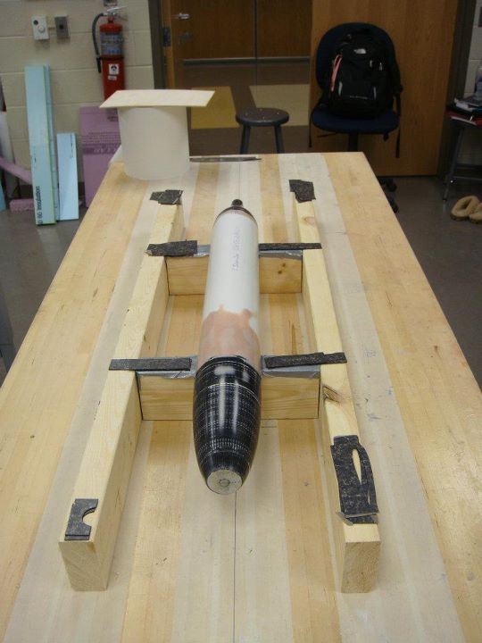
Once the printing was complete the seniors took over the process.  First an internal frame was cut to support, center, and join the cone to the PVC pipe.  The cone was then filled with plaster of paris to support the surface. Bondo and spackle were then applied to the surface to fill any cracks. Team 4 also added a shaft that stuck out the end of the mold.  This was then attached to a jury-rigged lathe.  The shaft was removed and sanded smooth once its purpose was served.

Rough sanded plug

After hours of hard work the final plugs were completed.  The final sanded surface is so smooth that reflections are clearly seen on its surface.

Final plug

With the plugs complete the teams used wax and PVA to prepare the plug for the mold layup.  While team 4 did not have any trouble getting the plug out of the completed mold, team 3 did have some difficulties.  However, these difficulties have been attributed to the waxing and PVA processes and not the 3D printed PLA material.

Overall the experiment was successful in its goals of reducing time to create the plug and allowing for the creating of complex geometries.  In particular, sanding was reduced since only the final surface was sanded.  In the old process, sanding had to be done on the foam surface, fiberglass surface, and the painted surface all of which took time.  Additionally, the geometries would have been difficult to create by other methods. While team 4’s radially symmetric cones could have been created on a lathe, team3’s cones could not.  The success of this method should serve as a stepping stone for future designed using more complicated geometries.

Piccolo Telemetry Visualization

The Piccolo Command Center (PCC) software allows an operator to plan and execute flights using the Piccolo autopilot.  However, it can be difficult to analyze post-flight telemetry.  Additionally, access to the PCC software is limited.

To address this problem I created a matlab function “log2kml.m” to convert Piccolo log files into KML files readable by Google Earth (GE).  This function reads the space delimited log file into Matlab.  It then filters out bad GPS points.  Finally it steps through the data to create a KML polyline.  The line is segmented based on the flight mode to clarify what the autopilot was doing.  The function uses the KML toolbox created by Rafael Fernandes de Oliveira.  It can be found at http://www.mathworks.com/matlabcentral/fileexchange/34694.  This toolbox is put together well and was easy to use.

The results shown below make the high performance of the autopilot clear.  Since the points are 3D there is some distortion of the actual ground path.

AUVSI 2011 NCSU Competition Run

AUVSI 2011 NCSU Competition Run

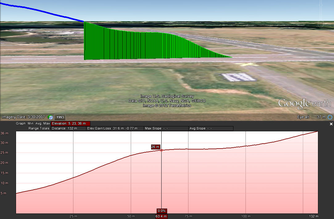
This visualization  allows us to analyze certain maneuvers much more easily.  A point of concern on autonomous take-offs has been a “dip” that occurs as the aircraft switches from prioritizing altitude to prioritizing airspeed.  Using the “Elevation Profile” tool in GE alongside the flight path allows for a clear observation of the performance.

Autonomous Take-off Performance

Autonomous Take-off Performance

It can now clearly be seen that the aircraft does level out, but does not lose altitude.  We can also determine that it levels off at an altitude of 21 meters or 68 feet above ground level.  This new knowledge can now be applied to improving future performance, or at least avoiding flying in to trees at the end of the runway.

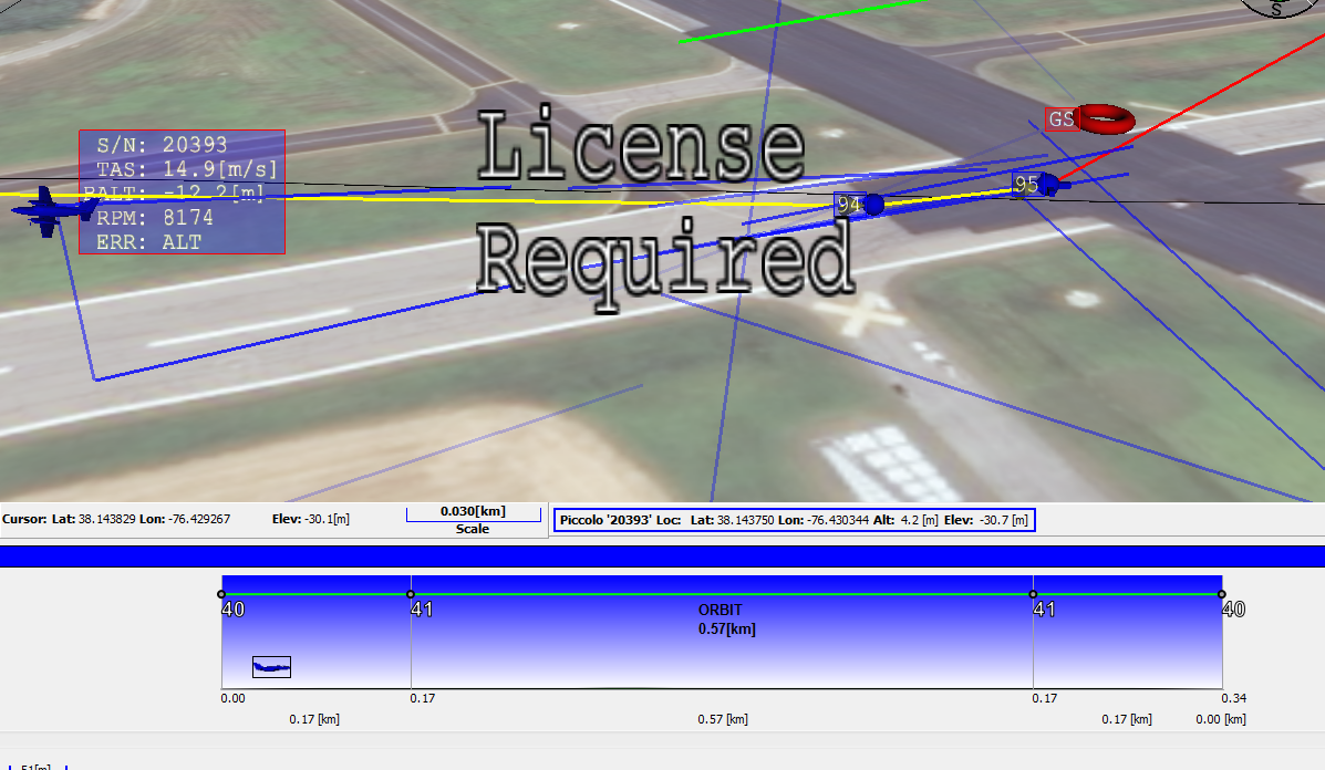
For comparison a screenshot from the PCC is shown below.  Since the blue line representing the flight path is so course, the fine motion of the aircraft is only apparent when animated.  The profile view only shows the current position of the aircraft.  Finally, the 3D view isn’t apart of the base software package resulting in the “License Required” text being splashed across the screen.

PCC View

PCC View

Return top